
EDA Project: Exploring Cannabis Data
The following post contains a collection of excerpts from a final project I worked on with Kevin McMorrow for the course, Exploratory Data Analysis, during my Junior year at Wesleyan. This project displays use of several data management and visualization techniques, as well as the statistical approach of Exploratory Factor Analysis. Additionally, I must express my gratitude for Professor Robert Kabacoff and his Exploratory Data Analysis course from which I learned many of these concepts and techniques.
Introduction
In recent years, Cannabis use has steadily moved away from the taboo and into the mainstream. Studies have shown promising results regarding the drug’s efficacy in treating a wide variety of ailments ranging from epilepsy to PTSD. With its increased acceptance, Marijuana has brought with it a plethora of interesting data. Consumer data, strain genealogy, and cannabinoid breakdowns have all proved to be valuable and interesting avenues for further research. In conducting this study, we hope to be able to further understand some of the technical jargon that surrounds the plant. More specifically, we hope to make sense of the relationships between Indica, Sativa, and Hybrid strains–and their respective effects. Additionally, we’d like to take a broad look at the dataset to get an idea of trends in the cannabis market.
Guiding Questions:
-
How do flavor and effect influence the user rating of a cannabis strain?
-
How do strain types (indica, hybrid, sativa) differ in terms of flavor and effect compositions?
-
Are there underlying factors within the data? If so, what are they?
Data Description
Our data was sourced from Kaggle, which is an aggregated dataset of information scraped from the website, Leafly.com. The dataset provides information such as strain type, rating, reported effect, reported flavor, and description, on 2,350 unique Cannabis strains. These variables are categorical with the exception of the rating variable, which is nominal.
Data Preprocessing
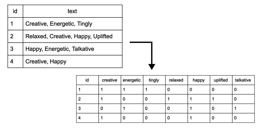
In terms of data management, we focused primarily on the variables, effect (strain effect) and flavor (strain flavor). Both variables in their raw format were composed of comma separated strings, which list each observation’s respective flavors and effects. To perform factor analysis, we converted these columns into two separate document term matrices, which displayed a binary (1,0) value for each strain, across each of the 13 unique effects and 49 unique flavors. The diagram below depicts an example of how the input and output of this transformation looks:
The code for our data management on the effects column is as follows:
## Replace commas with spaces
df$Effects <- gsub(",", " ", df$Effects)

## Create a corpus of text from the effects column:
library(tm)
df_corpus <- Corpus(VectorSource(df$Effects))

## Set text to lowercase
corpus_clean <- tm_map(df_corpus, tolower) # set text to lower

## Create document term matrix, then convert to a dataframe:
DTM <- DocumentTermMatrix(corpus_clean)
effects <- as.data.frame(as.matrix(DTM))
Exploratory Factor Analysis (EFA)
A Brief Introduction to EFA:
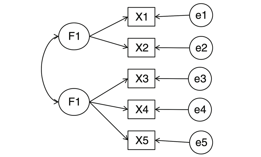
To reiterate, the Kaggle dataset includes an effects column and a flavors column, which contains 13 and 49 unique values, respectively. Considering the vast range of terms used to characterize the flavors and effects of these strains, we chose exploratory factor analysis because it “looks for a smaller set of underlying or latent constructs that can explain the relationships among the observed variables” (Kabacoff 2011). What EFA assumes is that there are underlying factors that “‘cause’ the observed variables” (Kabacoff 2011). In our case, these would be factors that underlie the 13 effects and 49 flavors observed in our dataset. The following diagram, provided by Professor Robert Kabacoff, depicts two underlying factors that are assumed to characterize the given variables, X1 through X5, with corresponding errors, e1 through e5, which represent the variances in X1 - X5 that cannot be explained through factors 1 and 2.
In EFA, factors are modeled from correlations among multiple variables. Additionally, EFA models assume that each factor explains the variance that is shared between two or more variables. Kabacoff uses the following formula as a representation of an EFA model:
\[X_1 = a_1 F_1 + a_2 F_2 + ... + a_p F_p + U_i\]…
\[X_k = a_1 F_1 + a_2 F_2 + ... + a_p F_p + U_i\]Where for every ith observed variable (i = 1…k), the common factors, $F_j$ contribute $a_i$ toward the composition of variable, $X_i$.
Running EFA on Cannabis Data:
Now onto the EFA model we ran on Kaggle’s cannabis data. The goal of exploratory factor analysis is to reduce the dimensionality of a given data set. In this case, there were 13 unique effects and 49 unique flavors. Our goal, by using EFA, was to explain the underlying latent factors of these variables to more clearly characterize the effect and flavor of the cannabis strains.
For the purposes of this blog post, I will only cover the process we undertook for cannabis effects, as working with the flavors was practically identical.
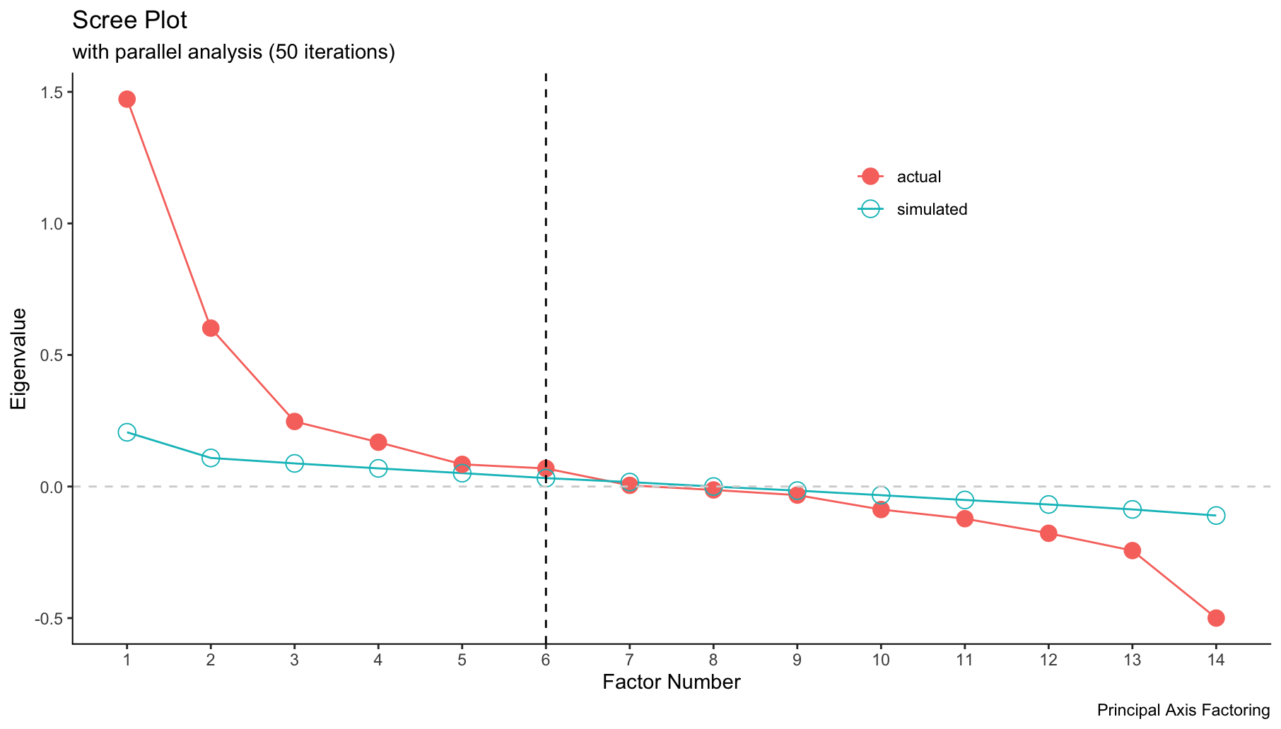
To start, we needed to choose how many factors could sufficiently describe the variance across the 13 effects. Scree plots are useful for this by displaying number of factors on the x-axis and their corresponding eigenvalues on the y-axis. The plot below depicts the scree plot for cannabis effects. The plot starts with the factor that explains the most variance among the effect variables and works its way down towards those that explain the least. In our case, the factors did not explain much of the variance in strain effects, which I will touch on when discussing the results. Furthermore, the scree plot below recommends the use of 6 factors, as the slope levels off around 5 or 6 factors, therefore the factors that are left out explain little to no variance among the effect variables (factors with eigenvalues below zero are almost always disregarded).
It is also important to note that the Kaiser-Harris criteria for scree plot cut off points is 0 when conducting exploratory factor analysis.
screePlot(strain_effect, method="pa")
Results:
For our EFA model, we used orthogonal varimax rotation, a commonly used rotation method implemented after factors are chosen. Varimax rotation chooses a factor rotation that maximizes the sum of variance explained by the common factors.
fit.effect <- FA(strain_effect, fm="pa", rotate="varimax", nfactors=5)
fit.effect
plot(fit.effect, type="bar")
Based on the total variance explained of our EFA model, the 5 factors we’ve chosen explain 29% of the variance in the original 13 effects variables. The column, h2, represents each variable’s communality. Communality measure the proportion of each variable’s variance that is explained by the common factors. This is also a sum of the squared factor loadings, which are individually displayed (F1 to F5). To better understand how varimax rotation helps us in determining what qualities our 5 factors are capturing, the visualization below depicts a before and after. As Kabacoff writes, this form of orthogonal rotation artificially your factors to be uncorrelated to one another. This makes interpreting our factors far easier:
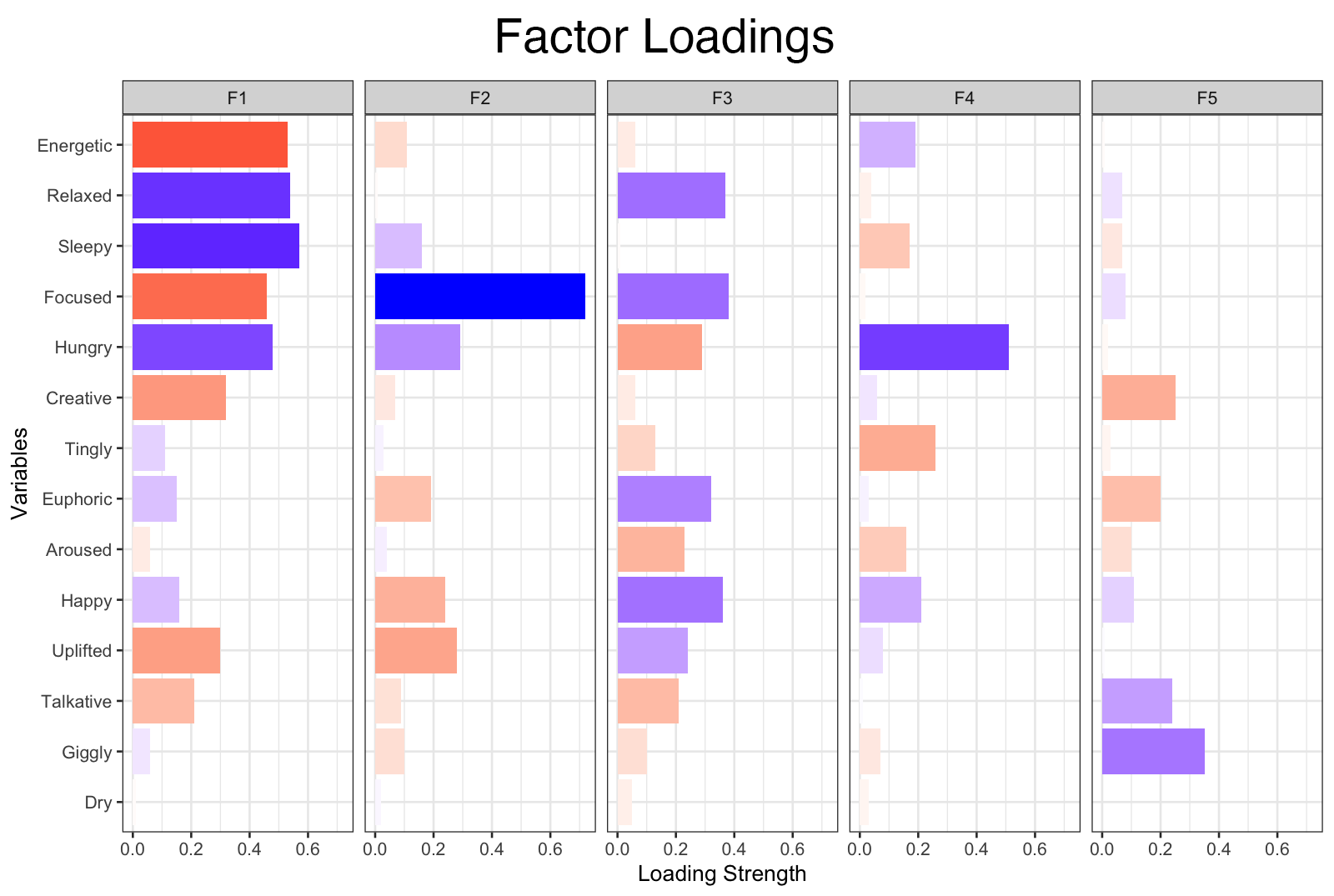

When rotated, the factor loadings for our EFA model showed much clearer correlations between each of the 13 effects and the 5 common factors. For example, “Focused” shows a strong, positive correlation with factor 2, “Hungry” shows a strong, positive correlation with factor 3, and “Energetic” shows a moderate, negative correlation with factor 1 (to name a few…). We used the loadings from our EFA model to inform how we labeled each factor, which can be seen below.
| Factor | Label |
|---|---|
| 1 | relaxing |
| 2 | focus |
| 3 | hunger |
| 4 | faded |
| 5 | solitary |
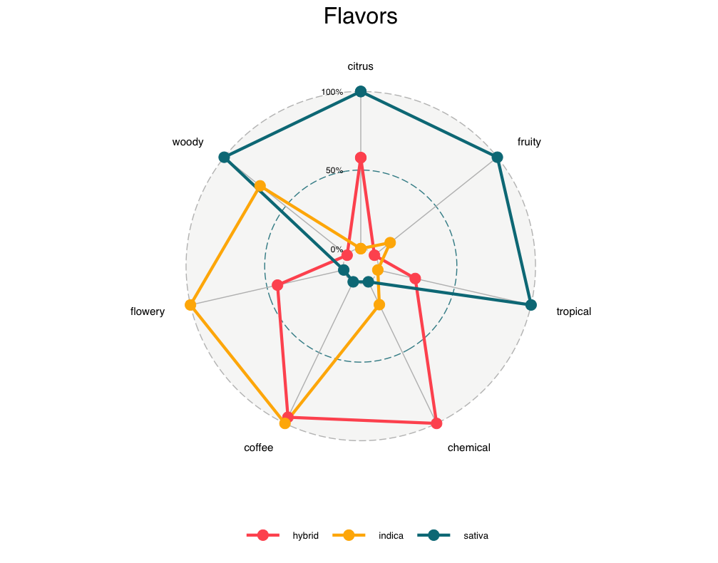
Visualizing the Factors from our EFA Analysis:
After labeling our factors, we visualized these across the three categories of strain type: indica, sativa, and hybrid. The example below shows a radar plot produced using the ggradar R package developed by Ricardo Bion. First, we summarized the data frame from our EFA analysis, computing the mean values of each factor across each of the three strain groups. We then rescaled these values to standardize the factors, resulting in the data frame, graph.data. The code below reflects this process for the cannabis effect factors, but the process for flavors is identical.
## Summarize data for graph
fa.effects %>%
  select(type, relaxing, focus, hunger,
         faded, solitary) %>%
  group_by(type) %>%
  summarise_if(is.numeric, funs(mean)) %>%
  mutate_at(vars(-type),
            funs(rescale)) -> graph.data

## Graph radar plot with graph data
library(ggradar)
library(scales)
ggradar(graph.data,
        grid.label.size = 4,
        axis.label.size = 4,
        group.point.size = 5,
        group.line.width = 1.5,
        legend.text.size= 10,
        legend.pos = "bottom") +
  labs(title = "Effects") +
  theme(plot.title = element_text(hjust = 0.5))

Discussion
Our findings (generally) fell within our expectations. The majority of strains caused happy & relaxed effects, and rarely evoked talkative or aroused feelings. Additionally, most strains exhibited “earthy” and “sweet” flavors. Through factor analysis, we were able to conclude that the effect and flavor profiles of hybrid strains fell neatly between indica and sativa strains–as was expected. Considering the increased acceptance of cannabis in the mainstream, our findings would likely have few implications for future policy. Instead, our research could have meaningful implications for market analysts, recreational/medicinal users, and dispensary owners. With the type of analyses that we conducted, individuals could easily find strains that are similar in effect, flavor, and user rating. Dispensaries could prioritize those strains with higher popularities, and search for similar cannabis strains to stock.
In regards to further research, we believe that an analysis of the user reviews could be both interesting, and valuable. Our dataset only provided the user ratings (on a scale from 1-5), despite there being thousands of lengthy strain-reviews left by Leafly users. These reviews could lend themselves to sentiment analysis. Additionally, we could use these reviews to extract the more nuanced effects, flavors, and attributes of the strains. For future research, we’re also interested in the chemical breakdown of these strains. Researchers have posited that strain-type (indica, sativa, hybrid) is an ineffective attribute to determine the effect/“personality” of a specific strain. Instead, it is suggested that one examines the cannabinoid makeup of a strain. The most important cannabinoids in determining the strain’s effects are THC (the psychoactive component) and CBD (the therapeutic/medicinal component). Getting ahold of this sort of data would be incredibly useful in our attempts to classify, summarize, and cluster large amounts of cannabis strains.
References
Kabacoff, R. (2011). R in Action, Second Edition. 2nd ed. Shelter Island, NY: Manning Publications.
Larsen, Liam. 2019. “Cannabis Strains”. Kaggle.com. https://www.kaggle.com/kingburrito666/cannabis-strains.