Machine Learning Project: Political Social Media Messages

12 minute read

The following includes a brief overview of a class project I worked on with Phillip Wong and Sangwon Kim at Wesleyan University (course: QAC385, Machine Learning). This project uses Naive Bayes as well as several data management and visualization techniques.

Problem Statement

As social media platforms such as Facebook and Twitter are becoming increasingly utilized in American politics, there exists a growing importance to understand the strategies and tactics employed by politicians through social channels. We’ve decided to undertake a project analyzing political social media posts. The following are several of the questions we posed prior to our analysis:

Can we predict the gender, age, and/or party of a given politician based on their social media posts?
Are there specific terms associated more strongly with a given party than others?
Can we use machine learning to interpret a given Independent poltician’s social media posts as either left leaning or right leaning?

Data Description

In order to tackle the questions outlined above, we used a combination of two datasets: Political Social Media Posts and U.S. Legislator Attributes.

The Political Social Media Posts dataset was obtained from Kaggle, but was originally sourced through CrowdFlower. The data was collected through numerous anonymous contributors, who looked at politician’s social media posts from December 31st, 2012 to December 30th, 2014. The anonymous contributors classified the dataset by qualitatively classifying the messages into audience (national or constituency) and bias (neutral/bipartisan or biased/partisan). The primary variable used from this set was text, which includes the text content of each social message.

The U.S. Legislator Attributes dataset was retrieved from GitHub. The database was aggregated from a variety of sources, but is maintained primarily by volunteers from well-known sources such as ProPublica and FiveThirtyEight. The collection of additional data has been automated, imported from additional sources, such as The Congressional Biographical Directory and C-SPAN’s Congressional Chronicle. The datasets we used were the Legislators Historical and Current datasets, which include all U.S. legislators from 1789 to present. The variables that we used for our analysis were age, party affiliation, gender and state affiliation of a given politician.

Data Preprocessing

Kaggle Data:

In terms of data preprocessing, we first dealt with missing observations by taking the column sums across our dataset. Only 4 of the 21 variables in our dataset contained missing values. Considering they were unimportant in terms of the analysis we were conducting, these columns were dropped accordingly.

Github Data:

First, we imported both the historical and current datasets on U.S. legislator attributes, subsetting the variables that would be important for our analysis (e.g. Full Name, Gender, Party, Bio ID, and Birthday). We then used rbind() to bind the rows of these two datasets so we could get a complete set of all U.S. legislators with their attributes. Finally we used a left_join to merge the data-managed legislator attributes to the Kaggle dataset.

Completed Data Set:

Once we had our full dataset, we were able to begin the necessary data preprocessing steps for analyzing the text content of politicians’ social media messages (“text” column). First we created a corpus from the text column of our dataset, which contains the text content of each politician’s social media message. To clean the text corpus we used the packages, tm and SnowballC to perform proper data management steps.

Set text to lowercase

corpus_clean <- tm_map(df_corpus, tolower)

Remove numbers

corpus_clean <- tm_map(corpus_clean, removeNumbers)

Remove stopwords (e.g. “a”, “and”, “but”, etc.)

corpus_clean <- tm_map(corpus_clean, removeWords, stopwords())

Remove punctuation

corpus_clean <- tm_map(corpus_clean, removePunctuation)

Strip unnecessary white spaces

corpus_clean <- tm_map(corpus_clean, stripWhitespace)

Stem the words (“learning” or “learned” => “learn”)
```
corpus_clean <- tm_map(corpus_clean, stemDocument)
```

After cleaning the text content of our data, we then converted our text corpus to a document term matrix, which creates columns for each individual term in our corpus and a corresponding frequency of references for each row of our initial data set (the Exploring Cannabis project provides a visualization of this process). From here we performed a 75/25 training/testing split on our document term matrix and on the relevant dependent variables for our ML model (e.g. gender, political party).

In building a machine learning model, general practice requires a division of your data into a training and testing set (75% training, 25% testing is a common split). We train the machine learning model with the training data and test its accuracy with the testing data.

# create training and testing datasets
politic_dtm_train <- politic_dtm[1:3750, ] # 75% of data in training
politic_dtm_test <- politic_dtm[3751:5000, ] # 25% of data in training

# collect labels (party affiliation)
politic_train_labels <- temp_full$party[1:3750]
politic_test_labels <- temp_full$party[3751:5000]

Furthermore, we decided to only include terms that occurred at least 5 unique messages within the document term matrix and converted word counts to 1’s and 0’s, rather than frequency of word use per row. This was a necessary step because Naive Bayes requires categorical predictors, e.g. word occurrence rather than word frequency, therefore we had to convert the word variables to “Yes” or “No” (1,0) factors.

# indicator feature for frequent words
politic_freq_words <- findFreqTerms(politic_dtm_train, 5)
# returns words that have appeared in at least 5 messages

# subset training and testing datasets to only include these words...
politic_dtm_freq_train <- politic_dtm_train[, politic_freq_words]
politic_dtm_freq_test <- politic_dtm_test[, politic_freq_words]

# convert counts to a factor
convert_counts <- function(x) {
  x <- ifelse(x > 0, 1, 0)
  x <- factor(x,
              levels = c(0,1),
              labels = c("No", "Yes"))
  return(x)
}

# apply convert_counts() to columns of the train/test data
politic_train <- apply(politic_dtm_freq_train, 2, convert_counts)
# when using the apply() function on matrices, 1 refers to rows, 2 refers to columns.
politic_test <- apply(politic_dtm_freq_test, 2, convert_counts)

Machine Learning Approach

We used the Naive Bayes technique to analyze the structured text dataset. The Naive Bayes model is the de facto standard for text classification, simply given the nature of the dataset’s properties. A text classification dataset has a large number of features that each have a small impact on the final outcome, but these variables combined can have a large impact. The Naive Bayes model with text classification uses the frequencies of the words as its features to classify an observation (in our case social media posts) into a category (such as political party, gender). Naive Bayes, if run on a single feature (word), works by calculating the probability that an observation is is in a specific category by multiplying the likelihood and prior probability and dividing it by the marginal livelihood. To explain these terms, consider an example trying to predict that an email is spam considering that it has the word “free” in its contents.

\[P(spam | “free”) = \frac{P(“free” | spam) * P(spam)}{P(“free”)}\]

The likelihood is the probability that an observation that is spam has the word “free”. The prior probability is the probability that an observation is spam. The marginal livelihood is the probability that an observation has the word “free”. This calculates the goal posterior probability which is the probability that given the word “free” an observation is spam. However, obviously text classification works with observations that have more than one word, and thus works with many features. Naive Bayes deals with multiple features (words) by assuming that all of the features are of equal importance and the features are independent of each other, i.e. the presence of one word does not affect the presence of other words (hence the term Naive). So, the Naive Bayes model simply multiplies the likelihood of features in the equations and divides it by the total marginal livelihood of the features to be able to offer a probability that a word is in a specific category given multiple features. This is a basic understanding of how the Naive Bayes model works on features for text classification into categories, and it is what we used to classify political social media posts into categories such as party and gender.

Results

Predicting Party from Social Media Messages

First, we trained a Naive Bayes machine learning model to classify the party (Democrat, Independent, Republican) of a given politician based on the content of their social media messages. We used the e1071 R-package to build our Naive Bayes machine learning models and caret to produce confusion matrices and relevant results.

set.seed(1234)
politic_classifier <- naiveBayes(politic_train, politic_train_labels, laplace = 1)

# evaluate performance of model
politic_test_pred <- predict(politic_classifier, politic_test)

confusionMatrix(politic_test_labels, politic_test_pred, positive = "Democrat")

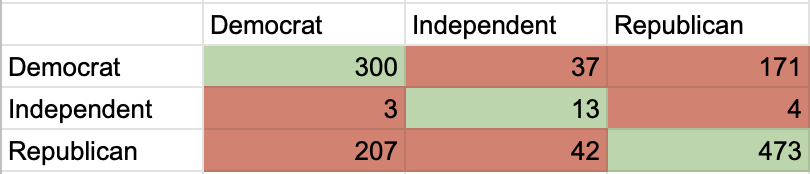
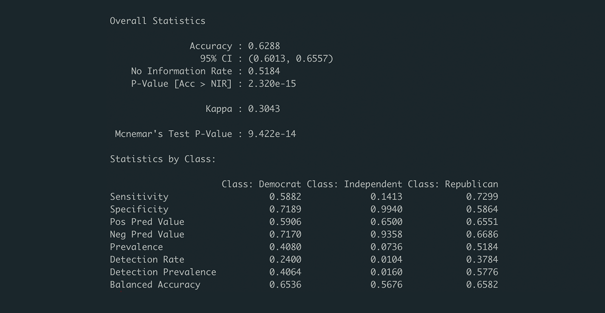
Our Naive Bayes model performed on the testing data with an accuracy of 0.6288 (classified 62.88% of the observations to the correct party). The sensitivities (proportion of actual positives that are correctly identified as such) were 0.5882 for Democrats, 0.7299 for Republicans, and 0.1413 for Independents. The specificities (proportion of actual negatives that are correctly identified as such) were 0.7189 for Democrats, 0.9940 for Independents, and 0.5864 for Republicans. Thus, more often than not, our model correctly predicted a social media post’s party, but was better at predicting if a Republican message was Republican and at knowing that a message was not Democratic.

We also trained and predicted on gender using the same Naive Bayes technique.

Predicting Gender from Social Media Messages

set.seed(1234)
gender_classifier <- naiveBayes(politic_train, gender_train_labels, laplace = 1)

# evaluate performance of model
gender_test_pred <- predict(gender_classifier, politic_test)

confusionMatrix(gender_test_labels, gender_test_pred, positive = "F")

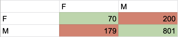
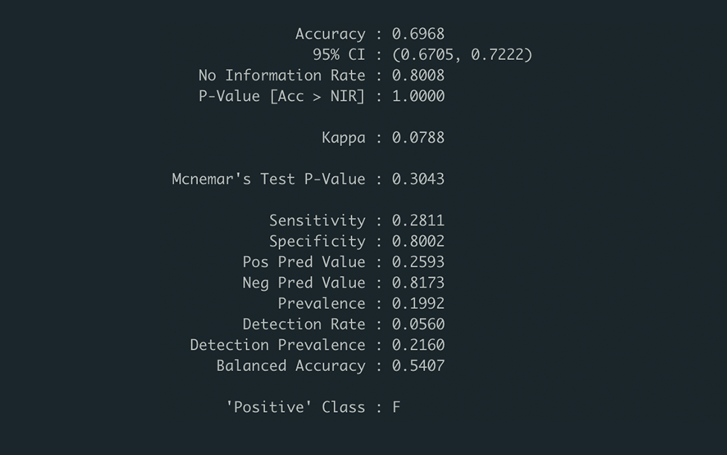
The model had an accuracy of 0.6968, and a sensitivity of 0.2811 and a specificity of 0.8002 when considering the “positive” class to be female. This means that it predicted about 70% of messages correctly, while predicting 80% of male messages correctly but only 28% of female messages correctly.

Supplemental Exploratory Analysis

Following our interpretation of the first Naive Bayes model, predicting political party, we decided to analyze the false negatives for the Independent party. By analyzing false negatives, we were able to see our model’s predicted probabilities for both Democrat and Republican on a given Independent politician’s social media messages. As an exploratory approach, the interpretation of false negatives was interesting as it could potentially articulate whether a given Independent’s message leaned more towards the left (Democratic) or towards the right (Republican).

After filtering by “Independent”, we discovered that the only politician in our testing set registered as an Independent was Bernie Sanders, therefore our initial hypothesis was that his false negative classifications would lean towards a larger predicted probability for Democrat than for Republican, as he is known to have more progressive, leftist politics.

party_predicted_probs <- as.data.frame(predict(politic_classifier, politic_test, type = "raw"))
party_predicted_probs <- round(party_predicted_probs, 4)

independent.compare <- cbind(party_predicted_probs, politic_test_labels, temp_full$full_name[3751:5000])

d <- which(independent.compare$politic_test_labels=="Independent" & independent.compare$Independent != 1)

independent.compare %>%
  filter(politic_test_labels == "Independent", Independent != 1) %>%
  cbind(temp_full$text[3751:5000][d]) -> independent.table

col.names.independent = c("Democrat", "Independent", "Republican",
                          "Party", "Name", "Text")

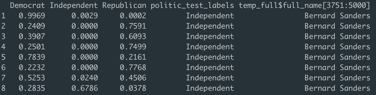
This table depicts our model’s predicted probabilities for our data’s single Independent candidate, Bernie Sanders (we omitted predictions of 1).

Naive Bayes works by having many features with small impacts coming together to have a large impact, but with these messages, there are so few words and features that just a few features are having large impacts, which goes against the foundational theory of Naive Bayes.

Examples of ‘low-feature’ messages: “Sign up to receive email updates from Sen. Sanders”, “Read Sen. Bernie Sanders’ progressive budget plan here”

For future analysis, it may be useful to use list-wise deletion or imputation on the DTM matrix by setting a row sum cutoff point. This could effectively ensure that the training/testing sets have more features per row to learn from.

Word Cloud: Frequencies of Democratic and Republican Term Usage

As a final exploratory data analysis technique, we decided to create a visualization showing terms frequently used by Democrats versus Republicans.

###### Comparison Cloud
cloud.words <-as.data.frame(as.matrix(politic_test))

cloud.words <- data.frame(apply(cloud.words, 2, function(x) {as.numeric(as.character(ifelse(x == "Yes", 1, 0)))}))

cloud.set <- cbind(politic_test_labels, cloud.words)

cloud.set.sums <- aggregate(cloud.set[2:1843], by = list(cloud.set$politic_test_labels), FUN = sum)

## Subset for words that occur more than 10 times:
cloud.freq.10 <- which(colSums(cloud.set.sums[-1])>10)
cloud.set.sums <- cloud.set.sums[,c("Group.1", names(cloud.freq.10))]

cloud.set.sums %>%
  gather(Term, Count, obamacar:howev) %>%
  filter(Group.1 != "Independent") -> cloud.set.key

cloud.data <- data.frame(Democrat = cloud.set.key[cloud.set.key$Group.1 == "Democrat",]$Count,
                         Republican = cloud.set.key[cloud.set.key$Group.1 == "Republican",]$Count,
                         row.names = unique(cloud.set.key$Term))

par(mfrow=c(1,1))
set.seed(1234)
comparison.cloud(as.matrix(cloud.data), random.order=FALSE, colors = c("lightsteelblue3","indianred3"),
                 title.size=2.5, max.words=400)

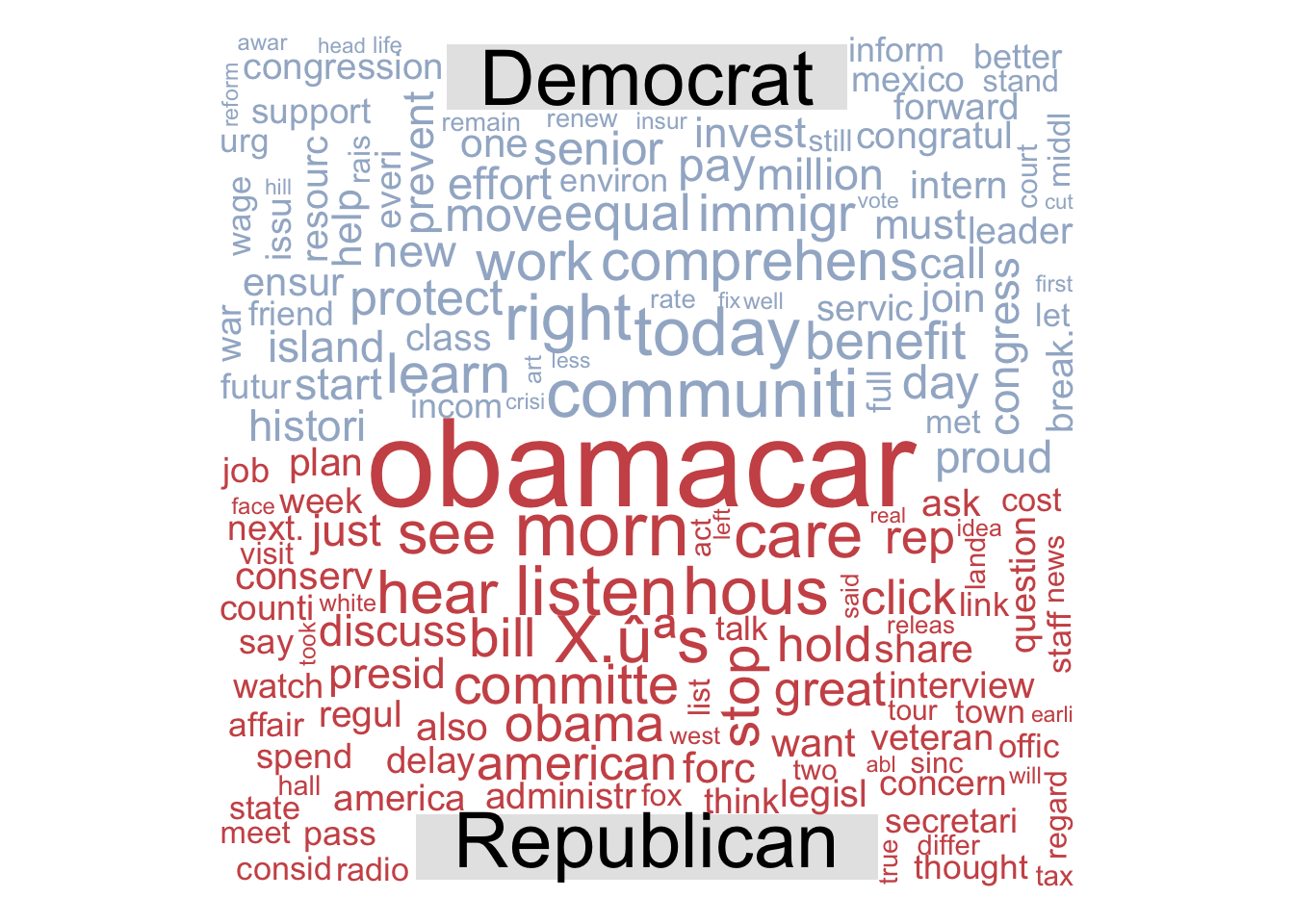
Word cloud for frequently used terms (Democrats vs. Republicans)

It is important to note that these terms have gone through stemming as well as other transformations to ensure homogeneity. - this accounts for the incompleteness of some terms.

Words that we found particularly interesting were “communities”, “immigration”, “equal”, “protect”, and “benefit” for Democrats and “conservative”, “pass”, “committee”, “stop”, and “fox” for Republicans. We found these terms interesting as they tend to align more closely with the ideologies of their respective parties. Additionally, many of the terms that appeared on either side of the word cloud often appear in the rhetoric articulated by politicians of the respective parties. One last term that we found interesting was the frequency of Republicans using the term “Obamacare”, considering this was a health care policy implemented under a Democratic presidency. For further research, a sentiment analysis could potentially show whether Republicans are using the term in a positive or negative tone (our hypothesis would most likely align with Republican sentiments being negative).

Discussion

Our model predicted relatively well in classifying political party, with an accuracy of 63%, it was better at correctly classifying Republican messages than Democrat ones. Additionally the model performed poorly on Independent messages, but this is most likely due to a heavy imbalance in Independent messages compared to Democrat and Republican messages. With nearly 2% of the training set being composed of Independent messages, we lacked sufficient data to produce a well-trained model for Independent classification.

For gender, our model performed better with an accuracy of almost 70%. It did very well in predicting male messages (80%), but poorly on predicting female messages (28%). Like the Independent party, this may be an effect of imbalanced classes (M/F). Furthermore, the imbalance in our data could also be a reflection of a gender imbalance in U.S. Congress.

We hope that our findings contribute to forming a better understanding of how the rhetoric of politicians changes across parties. From this, we can get a better sense of what policies/issues are important to different parties as well as what terms appear as heavily partisan. Additionally, our model can be used to highlight and classify super PAC, or other third-party party affiliations. Politicians can use this information in order to target individuals for various political purposes, such as soliciting donations or to target new members for their own personal constituencies.

In addition, our model can help politicians get a better understanding of what terms align more strongly with a certain political ideology. With this, they can structure their messages in a way that appeals more to a specific audience.

Furthermore, to best understand how the turn towards digital advertising has changed American politics, additional work could be done to analyze political messages through time. With a larger dataset, we could see how political rhetoric has changed over time, since the turn of digital advertising. We could also compare the rhetoric of digital advertising to that of television advertising. We would imagine that the rhetoric of digital advertising tends towards succinctness rather than breadth.

References

Kabakoff, Robert. “Naive Bayes.” Applications of Machine Learning in Data Analysis, 2 Oct. 2019. Wesleyan University. Lecture.

Share on

Twitter Facebook LinkedIn

Conner Sexton